The Complete Guide to Image Compression with OpenCV

In this tutorial, we will explore image compression, understand its theory, and learn how to perform it using OpenCV.

Image compression is a critical technology in computer vision that allows us to store and transmit images more efficiently while maintaining visual quality. Ideally, we’d love to have small files with the best quality. However, we must make the tradeoff and decide which is more important.

This tutorial will teach image compression with OpenCV, covering theory and practical applications. By the end, you’ll understand how to compress photos successfully for computer vision projects (or any other projects you might have).

What is Image Compression?

Image compression is reducing an image’s file size while maintaining an acceptable level of visual quality. There are two main types of compression:

1. Lossless compression: Preserves all original data, allowing exact image reconstruction.
2. Lossy compression: Discards some data to achieve smaller file sizes, potentially reducing image quality.

Why Compress Images?

If “disk space is cheap,” as we often hear, then why compress images at all? At a small scale, image compression doesn’t matter much, but at a large scale, it’s crucial.

For instance, if you have a few images on your hard drive, you can compress them and save a few megabytes of data. This is not much of an impact when hard drives are measured in Terabytes. But what if you had 100,000 images on your hard drive? Some basic compression saves real time and money. From a performance perspective, it’s the same. If you have a website with a lot of images and 10,000 people visit your website a day, compression matters.

Here’s why we do it:

• Reduced storage requirements: Store more images in the same space
• Faster transmission: Ideal for web applications and bandwidth-constrained scenarios
• Improved processing speed: Smaller images are quicker to load and process

Theory Behind Image Compression

Image compression techniques exploit two types of redundancies:

1. Spatial redundancy: Correlation between neighboring pixels
2. Color redundancy: Similarity of color values in adjacent regions

Spatial redundancy takes advantage of the fact that neighboring pixels tend to have similar values in most natural images. This creates smooth transitions. Many photos “look real” because there is a natural flow from one area to the other. When the neighboring pixels have wildly different values, you get “noisy” images. Pixels changed to make those transitions less “smooth” by grouping pixels into a single color, making the image smaller.

Color redundancy, on the other hand, focuses on how adjacent areas in an image often share similar colors. Think of a blue sky or a green field—large portions of the image might have very similar color values. They can also be grouped together and made into a single color to save space.

OpenCV offers solid tools for working with these ideas. Using spatial redundancy, OpenCV’s cv2.inpaint() function, for example, fills in missing or damaged areas of a picture using information from nearby pixels. OpenCV lets developers use cv2.cvtColor() to translate images between several color spaces regarding color redundancy. This can be somewhat helpful as a preprocessing step in many compression techniques since some color spaces are more effective than others in encoding particular kinds of images.

We’ll test out some of this theory now. Let’s play with it.

Hands on Image Compression

Let’s explore how to compress images using OpenCV’s Python bindings. Write out this code or copy it:

You can also get the source code here

import cv2
import numpy as np

def compress_image(image_path, quality=90):
    # Read the image
 img = cv2.imread(image_path)
    
    # Encode the image with JPEG compression
 encode_param = [int(cv2.IMWRITE_JPEG_QUALITY), quality]
 _, encoded_img = cv2.imencode('.jpg', img, encode_param)
    
    # Decode the compressed image
 decoded_img = cv2.imdecode(encoded_img, cv2.IMREAD_COLOR)
    
    return decoded_img

# Example usage
original_img = cv2.imread('original_image.jpg')
compressed_img = compress_image('original_image.jpg', quality=50)

# Display results
cv2.imshow('Original', original_img)
cv2.imshow('Compressed', compressed_img)
cv2.waitKey(0)
cv2.destroyAllWindows()

This example contains a compress_image function that takes two parameters:

• Image path (where the image is located)
• Quality (the quality of the image desired)

Then, we’ll load the original image into original_img. We then compress that same image by 50% and load it into a new instance, compressed_image.

Then we’ll show the original and compressed images so you can view them side by side.

We then calculate and display the compression ratio.

This example demonstrates how to compress an image using JPEG compression in OpenCV. The quality parameter controls file size and image quality tradeoff.

Let’s run it:

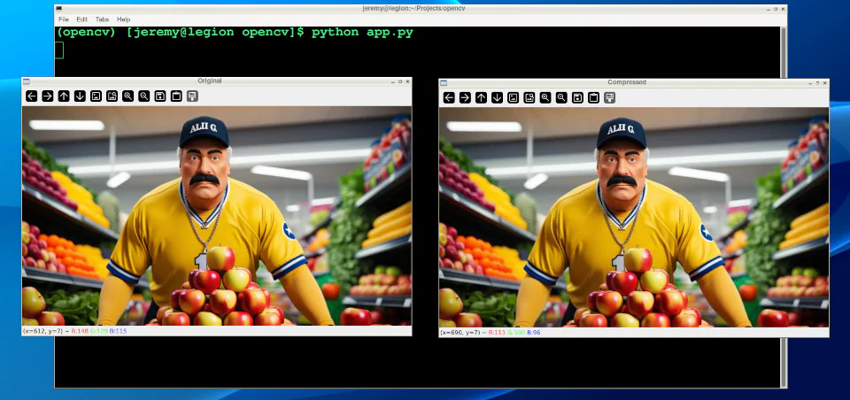
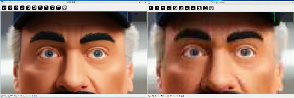
While initially looking at the images, you see little difference. However, zooming in shows you the difference in the quality:

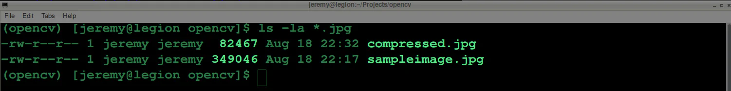
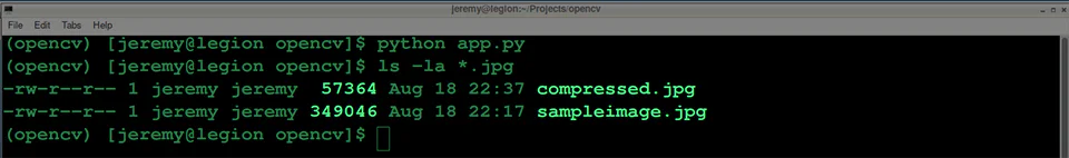
After closing the windows and looking at the files, we can see the file was reduced in size dramatically:

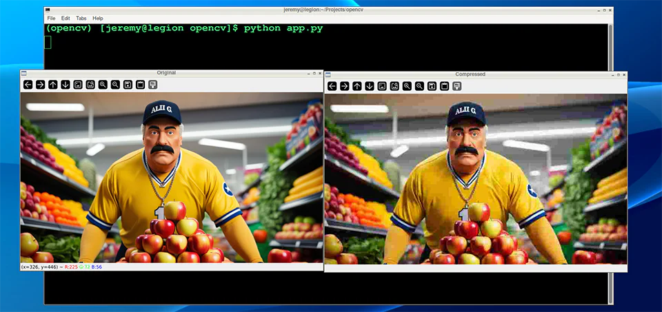
Also, if we take it down further, we can change our quality to 10%

compressed_img = compress_image('sampleimage.jpg', quality=10)

And the results are much more drastic:

And the file size results are more drastic as well:

You can adjust these parameters quite easily and achieve the desired balance between quality and file size.

Evaluating Compression Quality

To assess the impact of compression, we can use metrics like:

1. Mean Squared Error (MSE)

Mean Squared Error (MSE) measures how different two images are from each other. When you compress an image, MSE helps you determine how much the compressed image has changed compared to the original.

It does this by sampling the differences between the colors of corresponding pixels in the two images, squaring those differences, and averaging them. The result is a single number: a lower MSE means the compressed image is closer to the original. In comparison, a higher MSE means a more noticeable loss of quality.

Here’s some Python code to measure that:

def calculate_mse(img1, img2):
    return np.mean((img1 - img2) ** 2)

mse = calculate_mse(original_img, compressed_img)
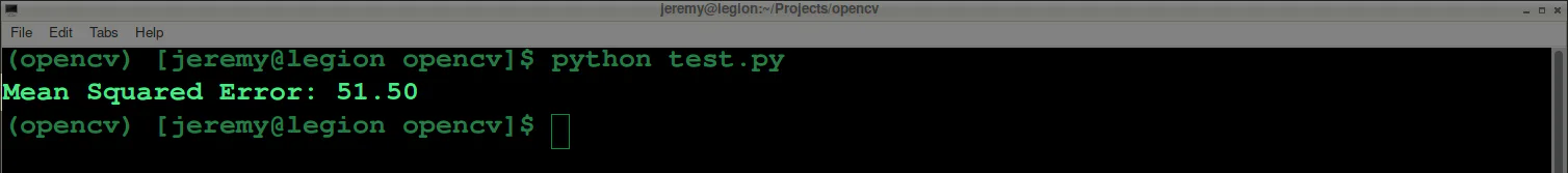
print(f"Mean Squared Error: {mse:.2f}")

Here’s what our demo image compression looks like:

1. Peak Signal-to-Noise Ratio (PSNR)

Peak Signal-to-Noise Ratio (PSNR) is a measure that shows how much an image’s quality has degraded after compression. This is often visible with your eyes, but it assigns a set value. It compares the original image to the compressed one and expresses the difference as a ratio.

A higher PSNR value means the compressed image is closer in quality to the original, indicating less loss of quality. A lower PSNR means more visible degradation. PSNR is often used alongside MSE, with PSNR providing an easier-to-interpret scale where higher is better.

Here is some Python code that measures that:

def calculate_psnr(img1, img2):
 mse = calculate_mse(img1, img2)
    if mse == 0:
        return float('inf')
 max_pixel = 255.0
    return 20 * np.log10(max_pixel / np.sqrt(mse))

psnr = calculate_psnr(original_img, compressed_img)
print(f"PSNR: {psnr:.2f} dB")

Here’s what our demo image compression looks like:

“Eyeballing” your images after compression to determine quality is fine; however, at a large scale, having scripts do this is a much easier way to set standards and ensure the images follow them.

Let’s look at a couple other techniques:

Advanced Compression Techniques

For more advanced compression, OpenCV supports various algorithms:

1. PNG Compression:

You can convert your images to PNG format, which has many advantages. Use the following line of code to set your compression from 0 to 9, depending on your needs. 0 means no compression whatsoever, and 9 is the maximum. Remember that PNGs are a “lossless” format, so even at maximum compression, the image should remain intact. The big tradeoff is file size and compression time.

Here is the code to use PNG compression with OpenCV:

cv2.imwrite('compressed.png', img, [cv2.IMWRITE_PNG_COMPRESSION, 9])

And here is our result:

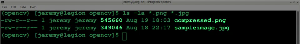
Note: You may notice sometimes that PNG files are larger, depending on the image.

1. WebP Compression:

You can also convert your images to .webp format. This is a newer method of compression that’s gaining in popularity. I have been using this compression on the images on my blog for years.

In the following code, we can write our image to a webp file and set the compression level from 0 to 100. It’s the opposite of PNG’s scale because 0, because we’re setting quality instead of compression. This small distinction matters, because a setting of 0 is the lowest possible quality, with a small file size and significant loss. 100 is the highest quality, which means large files with the best image quality.

Here’s the Python code to make that happen:

cv2.imwrite('compressed.webp', img, [cv2.IMWRITE_WEBP_QUALITY, 80])

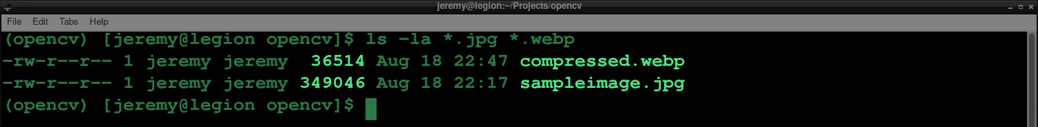
And here is our result:

These two techniques are great for compressing large amounts of data. You can write scripts to compress thousands or hundreds of thousands of images automatically.

Conclusion

Image compression is fantastic. It’s essential for computer vision tasks in many ways, especially when saving space or increasing processing speed. There are also many use cases outside of computer vision anytime you want to reduce hard drive space or save bandwidth. Image compression can help a lot.

By understanding the theory behind it and applying it, you can do some powerful things with your projects.

Remember, the key to effective compression is finding the sweet spot between file size reduction and maintaining acceptable visual quality for your application.

Thanks for reading, and feel free to reach out if you have any comments or questions!